Abstract
Gray leaf spot (GLS) is a fungal disease of maize (Zea mays) caused by Cercospora zeae-maydis and Cercospora zeicola. In laboratory settings, fungal isolates are grown on petri dishes and photographed at successive time points to characterise colony expansion, morphology, and structural organisation. Manual measurement of these traits is time-consuming and operator-dependent.
grayleafspotr provides a fully automated pipeline for
quantitative phenotyping of GLS colonies from time-lapse plate
photographs. The package uses a bundled SmallUNet deep-learning
segmentation model to identify colonies in each image, then extracts
morphometric and texture features that describe colony growth, shape,
and internal organisation over time. The resulting tidy data frame can
be explored with included template ggplot2 visualisations
or passed to any downstream R analysis.
Python dependencies are managed automatically through
basilisk; no manual Python environment setup is
required.
1. Package overview
What the package does
Given a folder of plate photographs, grayleafspotr:
- Detects the petri dish boundary using classical circle fitting.
-
Segments the colony inside the dish with a
SmallUNet model (
best_area_w_0.7.pt). - Extracts per-image features: area (mm²), equivalent diameter, circularity, eccentricity, edge roughness, crack coverage, texture entropy, and a radial intensity profile.
-
Returns a tidy result object — a
grayleafspot_run— containing a data frame indexed by filename and imaging day. -
Provides template plots — one function per figure,
all returning
ggplot2objects ready for further customisation.
Input requirements
| Requirement | Detail |
|---|---|
| Image formats | JPEG, PNG, BMP, TIFF, WEBP |
| Naming convention | Encode the day with a d\d+ token:
*_d04_*.jpg for day 4 |
| Plate diameter | Standard 90 mm (adjustable via plate_diameter_mm) |
| Folder structure | One folder per experiment; one image per plate per time point |
Example filenames and the day values they produce:
20260210_P001_06-FEB_WT_PCBM_SUB_d04_TOP.jpg  →  day 4
20260212_P001_06-FEB_WT_PCBM_SUB_d06_TOP.jpg  →  day 6
20260216_P001_06-FEB_WT_PCBM_SUB_d10_TOP.jpg  →  day 10
Workflow at a glance
Plate images (folder)
        │
        ▼
grayleafspot_analyze()  /  grayleafspot_run()
        │
        ├─ Dish geometry detection  (classical Hough transform)
        ├─ SmallUNet segmentation   (best_area_w_0.7.pt)
        └─ Feature extraction       (area, shape, texture, cracks, radial)
        │
        ▼
grayleafspot_run S3 object
        │
        ├─ $results   per-image feature data frame
        └─ $run       run manifest (paths, timestamp, engine)
        │
        ▼
Template ggplot2 plots  /  tidy data  /  custom analysis
2. Installation
Install from Bioconductor:
if (!requireNamespace("BiocManager", quietly = TRUE))
    install.packages("BiocManager")
BiocManager::install("grayleafspotr")
Python dependencies (NumPy, OpenCV, PyTorch, scikit-image, etc.) are
installed automatically by basilisk the first time the
analysis pipeline is invoked. This one-time setup may take a few
minutes; subsequent calls use the cached environment instantly.
3. Bundled example data
The package ships three pre-computed example results so that all plotting and data-wrangling functions can be explored without running the full pipeline.
3.1 Load the example run
example_run <- example_grayleafspot_results()3.2 Inspect the feature table
example_run$results[, c("filename", "day", "area_mm2", "diameter_mm",
                         "circularity", "crack_coverage_pct", "qc_status")]
## # A tibble: 2 × 7
## filename day area_mm2 diameter_mm circularity crack_coverage_pct qc_status
## <chr> <dbl> <dbl> <dbl> <dbl> <dbl> <chr>
## 1 demo_day1… 1 12 3.9 0.8 0 pass
## 2 demo_day2… 2 18 4.78 0.77 2.5 pass3.3 Locate bundled source images
The three plate photographs used to generate this example are also
included in the package and are accessible via
system.file():
image_dir <- system.file("extdata", "testdata", "06FEB", package = "grayleafspotr")
list.files(image_dir)
## [1] "20260210_P001_06-FEB_WT_PCBM_SUB_d04_TOP.jpg"
## [2] "20260212_P001_06-FEB_WT_PCBM_SUB_d06_TOP.jpg"
## [3] "20260216_P001_06-FEB_WT_PCBM_SUB_d10_TOP.jpg"4. Template visualisations
Every plotting function accepts a grayleafspot_run
object and returns a ggplot2 object that can be customised
with standard ggplot2 calls.
Colony expansion over time
Colony equivalent diameter (mm) plotted against imaging day.
plot_colony_expansion(example_run)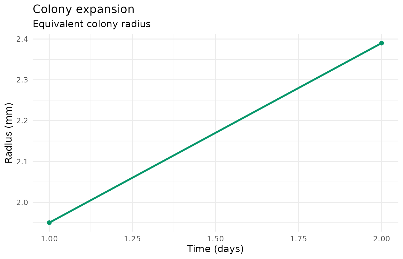
Growth rate and edge roughness
Daily growth increment (mm/day) alongside a measure of colony edge irregularity.
plot_growth_roughness(example_run)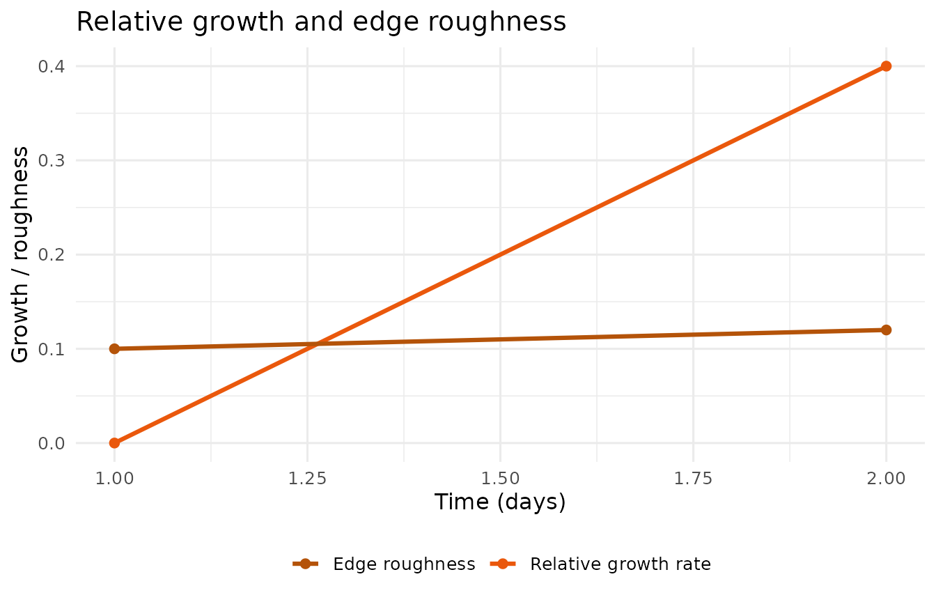
Crack coverage and count
Proportion of the colony mask classified as cracked tissue, alongside the total crack count — a proxy for structural stress.
plot_stress_remodeling(example_run)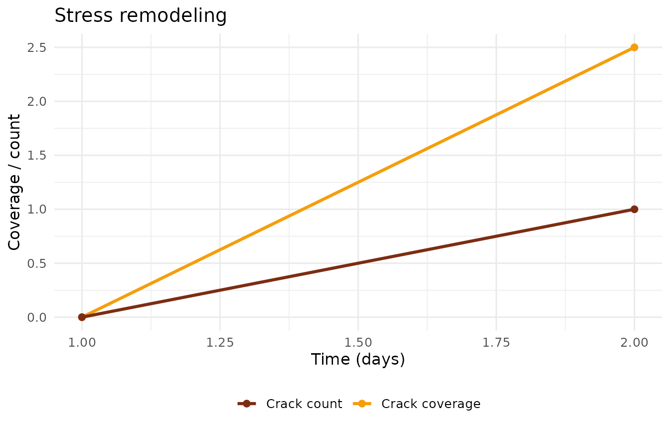
Texture organisation
Texture entropy and the centre-to-edge entropy gradient reflect internal colony heterogeneity.
plot_texture_organization(example_run)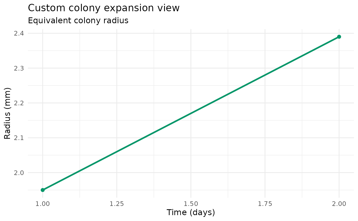
Shape versus stress
Eccentricity (0 = circular, 1 = elongated) plotted against crack coverage to reveal coupling between morphology and structural remodelling.
plot_shape_vs_stress(example_run)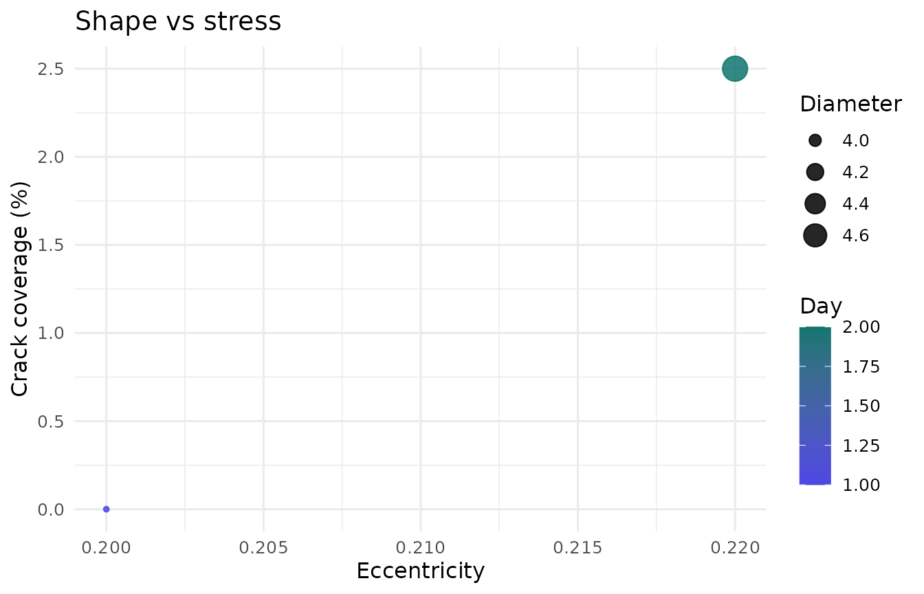
Feature correlation heatmap
Pearson correlations between all numeric features.
plot_feature_heatmap(example_run)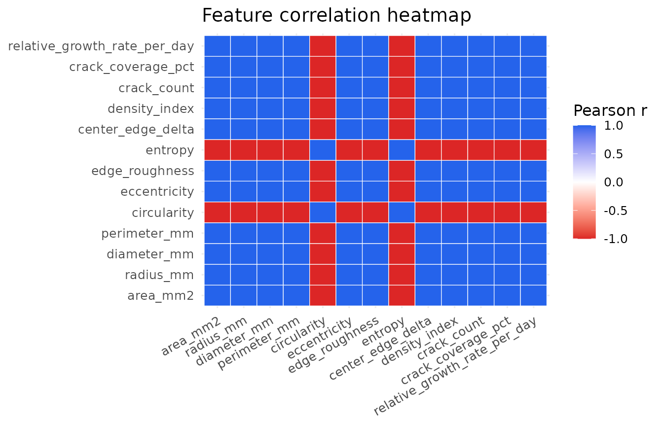
Radial intensity profile
Mean pixel intensity as a function of normalised radial distance from the colony centre.
plot_radial_profile(example_run)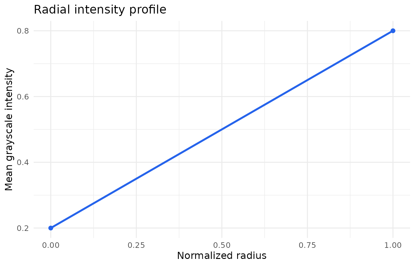
5. Work with tidy data
Convert the run object to a plain data frame for any downstream workflow:
growth_data <- as_grayleafspot_growth_data(example_run)
growth_data
## # A tibble: 2 × 34
## id filename day area_mm2 radius_mm diameter_mm perimeter_mm circularity
## <chr> <chr> <dbl> <dbl> <dbl> <dbl> <dbl> <dbl>
## 1 demo-1 demo_day… 1 12 1.95 3.9 8 0.8
## 2 demo-2 demo_day… 2 18 2.39 4.78 9.1 0.77
## # ℹ 26 more variables: eccentricity <dbl>, edge_roughness <dbl>,
## # contrast <dbl>, correlation <dbl>, energy <dbl>, homogeneity <dbl>,
## # entropy <dbl>, center_edge_delta <dbl>, density_index <dbl>, core <dbl>,
## # middle <dbl>, outer <dbl>, crack_count <dbl>, crack_length_mm <dbl>,
## # crack_coverage_pct <dbl>, proportional_crack_coverage_pct <dbl>,
## # radial_velocity_mm_per_day <dbl>, area_growth_rate_mm2_per_day <dbl>,
## # relative_growth_rate_per_day <dbl>, radial_acceleration <dbl>, …Custom plot
Because every template function returns a ggplot2
object, you can layer on additional components:
plot_colony_expansion(example_run) +
  ggplot2::labs(
    title    = "Colony expansion — 06-FEB experiment",
    subtitle = "WT strain, PCBM substrate"
  ) +
  ggplot2::theme_classic()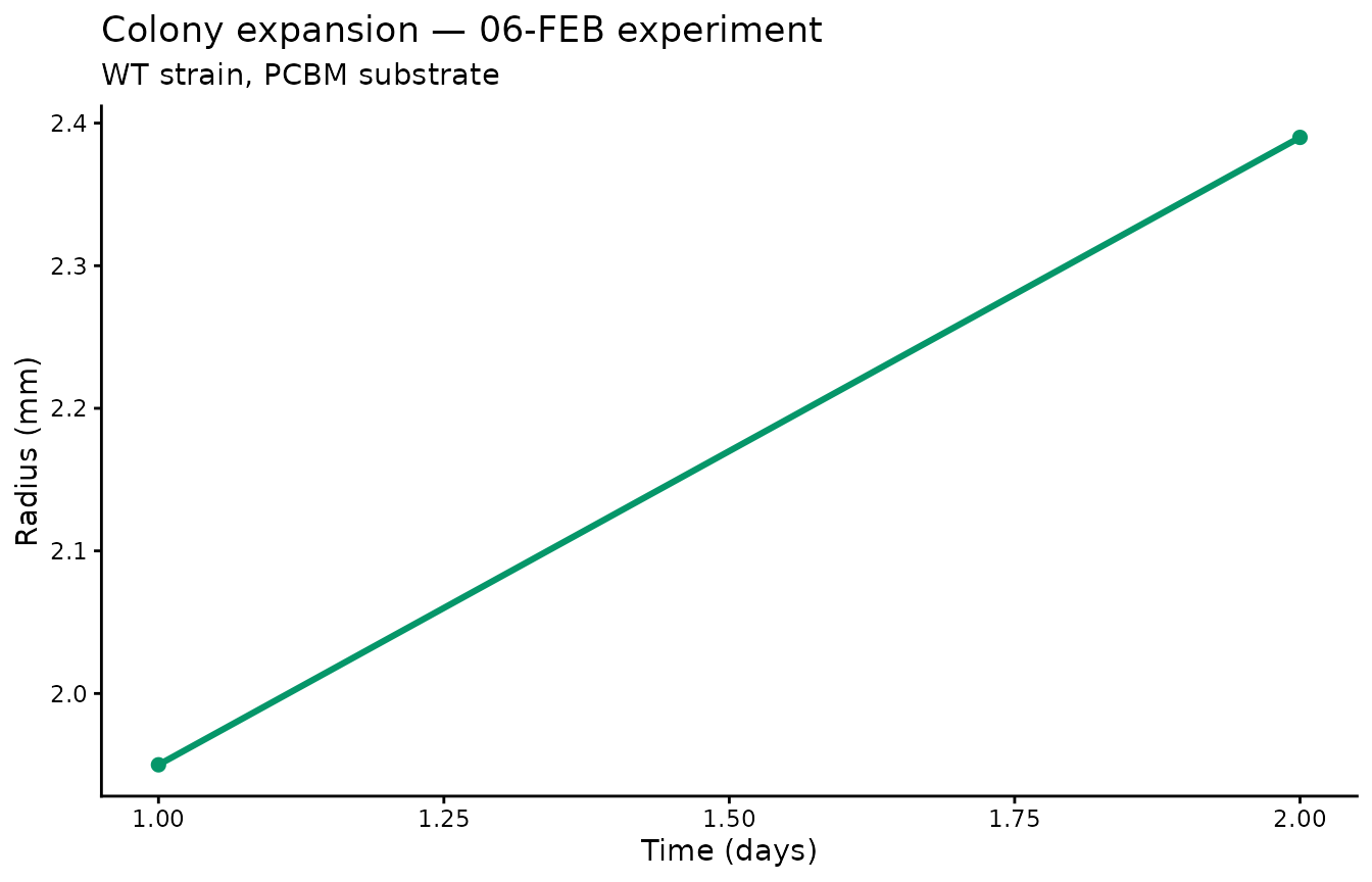
6. Analyze your own images
6.1 Prepare your image folder
Place all plate photographs for one experiment in a single directory.
The filename must contain a d\d+ token that encodes the
imaging day:
my_experiment/
├── isolate_A_d03_rep1.jpg
├── isolate_A_d05_rep1.jpg
├── isolate_A_d07_rep1.jpg
└── ...
6.2 Run the analysis — simple entry point
grayleafspot_run() is the recommended entry point for
most users. It returns the raw JSON payload as a named list.
res <- grayleafspot_run(
  input_dir  = "my_experiment",
  output_dir = "outputs",
  run_name   = "isolate_A"
)

res$results   # per-image feature table (data frame)
res$run       # run manifest
6.3 Full-featured alternative:
grayleafspot_analyze()
grayleafspot_analyze() returns a
grayleafspot_run S3 object with direct access to the
template plots:
run <- grayleafspot_analyze(
  input_dir  = "my_experiment",
  output_dir = "outputs",
  run_name   = "isolate_A"
)

plot_colony_expansion(run)
Why are these chunks not evaluated? They require actual plate images on disk and invoke the Python pipeline, which cannot run during package build. The executable examples in sections 3–5 above use the bundled pre-computed results and demonstrate the same data structures and plotting functions.
6.4 Reload saved results
Every run writes outputs to a timestamped sub-folder. Reload a previous run without re-running the pipeline:
run <- read_grayleafspot_results("outputs/20260427T142731Z_localunet")
plot_colony_expansion(run)
7. Developer note: Python override
Normal users do not need to configure Python. Developers maintaining
a local virtual environment (e.g. rvenv_arm_311) can bypass
basilisk by setting:
# ~/.Rprofile — developer use only
Sys.setenv(GRAYLEAFSPOTR_PYTHON = "/path/to/rvenv_arm_311/bin/python")
When GRAYLEAFSPOTR_PYTHON is set, the pipeline uses that
interpreter directly instead of the basilisk-managed environment.
Session information
## R version 4.6.0 (2026-04-24)
## Platform: x86_64-pc-linux-gnu
## Running under: Ubuntu 24.04.4 LTS
##
## Matrix products: default
## BLAS:   /usr/lib/x86_64-linux-gnu/openblas-pthread/libblas.so.3
## LAPACK: /usr/lib/x86_64-linux-gnu/openblas-pthread/libopenblasp-r0.3.26.so;  LAPACK version 3.12.0
##
## locale:
##  [1] LC_CTYPE=C.UTF-8       LC_NUMERIC=C           LC_TIME=C.UTF-8
##  [4] LC_COLLATE=C.UTF-8     LC_MONETARY=C.UTF-8    LC_MESSAGES=C.UTF-8
##  [7] LC_PAPER=C.UTF-8       LC_NAME=C              LC_ADDRESS=C
## [10] LC_TELEPHONE=C         LC_MEASUREMENT=C.UTF-8 LC_IDENTIFICATION=C
##
## time zone: UTC
## tzcode source: system (glibc)
##
## attached base packages:
## [1] stats     graphics  grDevices utils     datasets  methods   base
##
## other attached packages:
## [1] grayleafspotr_0.99.2
##
## loaded via a namespace (and not attached):
##  [1] generics_0.1.4     sass_0.4.10        utf8_1.2.6         lattice_0.22-9
##  [5] hms_1.1.4          digest_0.6.39      magrittr_2.0.5     evaluate_1.0.5
##  [9] grid_4.6.0         RColorBrewer_1.1-3 fastmap_1.2.0      jsonlite_2.0.0
## [13] Matrix_1.7-5       scales_1.4.0       textshaping_1.0.5  jquerylib_0.1.4
## [17] cli_3.6.6          rlang_1.2.0        crayon_1.5.3       bit64_4.8.2
## [21] withr_3.0.2        cachem_1.1.0       yaml_2.3.12        otel_0.2.0
## [25] tools_4.6.0        dir.expiry_1.20.0  parallel_4.6.0     tzdb_0.5.0
## [29] dplyr_1.2.1        ggplot2_4.0.3      filelock_1.0.3     basilisk_1.24.0
## [33] reticulate_1.46.0  vctrs_0.7.3        R6_2.6.1           png_0.1-9
## [37] lifecycle_1.0.5    fs_2.1.0           htmlwidgets_1.6.4  bit_4.6.0
## [41] vroom_1.7.1        ragg_1.5.2         pkgconfig_2.0.3    desc_1.4.3
## [45] pkgdown_2.2.0      bslib_0.11.0       pillar_1.11.1      gtable_0.3.6
## [49] glue_1.8.1         Rcpp_1.1.1-1.1     systemfonts_1.3.2  xfun_0.58
## [53] tibble_3.3.1       tidyselect_1.2.1   knitr_1.51         farver_2.1.2
## [57] htmltools_0.5.9    labeling_0.4.3     rmarkdown_2.31     readr_2.2.0
## [61] compiler_4.6.0     S7_0.2.2